Research

I build interpretable machine learning methods for modeling how people learn and how real-world systems behave, from student knowledge to traffic on the road.

Research interests

One question runs through my work: how is knowledge represented, both in the minds of learners and inside the models we build to understand them? I started by modeling what students know, which led me to ask what language models themselves "know." That in turn made me curious whether we can reach inside a model and change what it does. Along the way, I apply the same habits of careful, interpretable modeling to real-world systems like transportation.

Student modeling and cognitive science

A good student model should do more than predict right or wrong answers. It should describe what a learner understands, where their misconceptions are, and how that knowledge is organized. I am drawn to cognitive science for this reason: theories of how people learn, reason, and make errors give student models a structure that pure curve-fitting lacks. In Persona-MCMC, I represented each student as a readable natural-language persona that an LLM can use to predict answers to questions it has never seen. Next, I want to ground personas like these in cognitive theory, so they capture why a student answers the way they do, not only how often they are correct.

Understanding the core of the transformer

Using LLMs to model students raised a deeper question for me: what do these models actually represent internally? Attention is the core mechanism of the transformer. Each token builds its meaning from a weighted mix of the tokens around it. When I fine-tuned BERT to grade student science answers, I visualized its attention and found that it focused on content words in the question but did not clearly separate correct from incorrect answers. Attention alone did not explain the model's decisions. I want to understand the mechanisms underneath: how concepts are encoded in hidden layers, how information flows from layer to layer, and which components cause a given behavior.

Activation steering: from understanding to control

If concepts live as directions in a model's activation space, we can test that claim by intervening. Activation steering adds or removes such a direction during the forward pass and measures how the outcome changes. I find this exciting for two reasons. Scientifically, it turns interpretability from correlation into causal evidence: if steering a "misconception" direction changes the answers, the model really uses it. Practically, it could let us shape model behavior precisely, for example simulating a student with a specific misconception, or making an AI tutor more faithful to a learner's level, without retraining.

Probabilistic and interpretable AI

Across these questions, I prefer methods that show their reasoning. Persona-MCMC combines Markov chain Monte Carlo with language models so that each step of refinement is an explicit, inspectable proposal that is accepted or rejected. I want to keep pairing Bayesian thinking with interpretability, so that models are both accurate and understandable to the people who rely on them.

Machine learning for transportation systems

At the UF Transportation Institute, I apply the same mindset to infrastructure. Agencies cannot count traffic everywhere, so I build models that estimate intersection turning movement counts and Annual Average Daily Traffic (AADT) from the data that is available. I also build geospatial and computer vision pipelines that link map locations to the right roadway and read traffic values from map images. I care about honest evaluation: how well estimates generalize to new places, and how much each one can be trusted.

Computational modeling across disciplines

My background spans robotics motion planning applied to protein–ligand binding, and agent-based models of fractal polymer growth. These projects shaped how I work: borrow a strong method from one field, adapt it carefully to another, and benchmark it against the tools practitioners already trust.

Projects

Interpretable AI · Education

Persona-MCMC: Iterative LLM Persona Refinement for Interpretable Student Modeling

ML4ED Lab, UMass Amherst · Jun 2025 – Feb 2026 · with A. Scarlatos, H. McNichols & A. Lan · Manuscript in preparation for AIED 2027

Classical student models such as Item Response Theory summarize a student with a number. That number cannot say what the student knows, and it cannot be used for new questions. Persona-MCMC represents each student instead with a persona: a short, human-readable description of their strengths and weaknesses. A large language model then uses the persona to predict how the student will answer questions it has never seen.

To find a good persona, one LLM agent proposes small edits to the persona and another predicts the student's answers with it. Each edit is accepted or rejected using a Metropolis-Hastings-style rule based on predictive accuracy. Finally, an aggregation agent merges the top personas into one. On real student responses to math questions (NeurIPS 2020 Education Challenge), Persona-MCMC outperformed IRT and in-context learning baselines and produced personas that are more specific and topic-aware.

Method: Multi-agent LLM prompting (GPT-4.1-mini); Metropolis-Hastings-inspired acceptance with annealed temperature; top-K persona aggregation; comparison against 1PL IRT and in-context learning (ICL).

Left: the iterative refinement loop. Right: test-set accuracy and AUC from the paper (20 students, NeurIPS 2020 Education Challenge data). For ICL, accuracy and AUC are both ≈0.62, so the two dots overlap.

Transportation · Ongoing

Location-Based AADT Retrieval with Geospatial Matching

McTrans Center, University of Florida · Aug 2026 – Present

AADT (Annual Average Daily Traffic) is the average number of vehicles that use a road segment per day over a year. It is one of the most widely used inputs in transportation planning, safety analysis, and design. Getting the right AADT for a spot someone clicks on a map is harder than it sounds. Nearby roads, parallel facilities, intersections, and inconsistent data sources make it easy to match to the wrong segment.

I am building a pipeline that takes geographic coordinates, queries transportation data sources through GIS APIs, and uses roadway geometry to match the location to the correct roadway segment or intersection before retrieving its traffic data. I am also testing computer vision and OCR methods to extract and cross-check traffic values printed on transportation maps, with the aim of integrating the pipeline into production transportation software.

Method: Python geospatial processing; GIS APIs; spatial roadway and intersection matching; computer vision and OCR for map data extraction and validation.

How the pipeline works (schematic). A selected point is snapped to the roadway segment it belongs to, using distance and road geometry, before the segment's AADT is retrieved. A separate computer vision / OCR branch reads traffic values from map images to validate the result.

Transportation · Ongoing

Machine Learning Estimation of Intersection Turning Movement Counts

I-Street, UF Transportation Institute · Aug 2026 – Present

Turning movement counts (TMCs) record how many vehicles turn left, go straight through, or turn right on each approach of an intersection. They are essential for signal timing, capacity analysis, and intersection design. But collecting them requires field counts or video at each site, so most intersections have none.

I am developing a machine learning approach that estimates TMCs from traffic and roadway data that are already available. The work covers data processing, feature development, model evaluation, and analysis of where the estimates are reliable and where they are not.

Method: Data processing and feature engineering from traffic and roadway data; supervised machine learning; model evaluation and error analysis.

Left: a four-leg intersection has 12 turning movements (left, through, right on each approach). Right: the estimation problem. The model fills in this table for intersections that have no field counts.

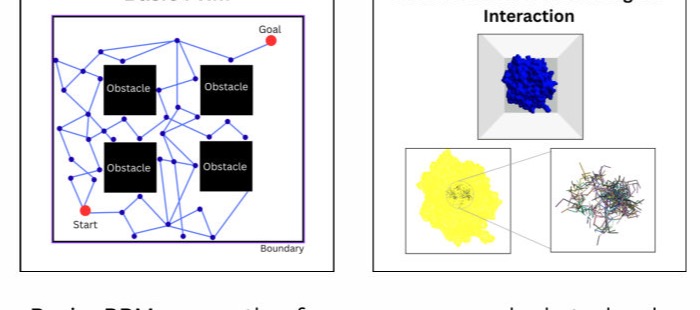
Basic probabilistic roadmap around obstacles, and the modified version sampling ligand poses around a protein

Robotics · Computational Biology

Protein–Ligand Affinity Score Using Motion Planning

RoSE Lab, Mount Holyoke & Parasol Lab, UIUC · Jun 2024 – Dec 2025 · with R. Mozumdar & D. Uwacu

For a drug molecule (ligand) to work, it must both reach a protein's binding site through an access tunnel and fit there in a low-energy pose. Standard tools like AutoDock and CAVER often ignore ligand size, flexibility, or energy along the way. We adapted a Probabilistic Roadmap (PRM), a robot motion-planning algorithm, to sample ligand configurations in a sphere around the active site. We scored each sample with an energy function to map the energy landscape, then compared the poses with AutoDock's. The sampled poses clustered consistently near the binding pocket (RMSD 6.25–6.97 Å to AutoDock poses).

Method: Modified PRM sampling (Parasol Planning Library); van der Waals / electrostatic energy evaluation; OpenMM molecular dynamics; benchmarking against AutoDock and CAVER; RMSD analysis.

View poster →

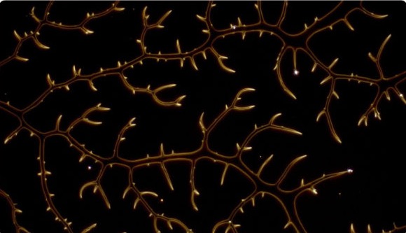
$Lab image of a branching poly(vinyl alcohol) fractal network$

Mathematical Modeling · Computer Vision

What if DLA Has It Backwards? Modeling Convergent Fractal Growth in Polymer Films

Dept. of Mathematics & Statistics, Hampshire College · Jan 2024 – May 2025 · with K. Mulder, C. Danese, M.-A. Bui, A. Nazhat & W. Chen · Pre-print

For 40 years, branching fractal patterns have been explained by Diffusion-Limited Aggregation (DLA), where branches grow outward and split apart from a seed. Our pre-print shows that poly(vinyl alcohol) films drying on a surface make the same-looking pattern in the opposite way. Across four drying methods (spin, center, sweep, and parallel), branches start and converge in the direction of flow. We introduce a triangular network model with a flow effect that reproduces this convergent growth consistently.

My part was building tools to parameterize and validate the model against lab images, which I presented at the Hudson River Undergraduate Mathematics Conference (HRUMC) 2025. I compared lab and simulated images with VGG-16 image embeddings: same-concentration model and lab images scored about 0.74 similarity at 99% concentration and 0.63 at 88%. I also turned images into skeleton networks in FIJI, wrote an algorithm to measure the angle at every branch junction, and compared lab and model angle distributions using KL divergence.

Method: Triangular agent-based growth simulation; VGG-16 embeddings with cosine similarity; FIJI/ImageJ preprocessing, binarization, and skeletonization; automated branch-angle algorithm; KL divergence.